

Mini-tutorial on statistical analysis: Correcting a common misinterpretation of p-values
Daniel Tancredi PhD, Professor of Pediatrics, UC Davis School of Medicine and Center for Healthcare Policy and Research, Sacramento, CA.
Decision makers frequently rely on p-values to decide whether and how to use a study to inform their decisions. Many misinterpret what a low p-value actually means, however. I will attempt to correct this common misinterpretation and explain how to use small p-values to evaluate whether a null hypothesis is plausible. I will show that a low p-value should be used in the same way that a clinician should use a valuable but imperfect clinical diagnostic test result; as one factor, but not the only one, on which to base a decision.
Typically, readers assume that if a p value is low, such as less than 0.05, and thus the test statistic is statistically significant at the conventional level, that there is a good chance that the study results are not “due to chance”. But it is not as simple as that. Let’s suppose that one has a p-value that was generated in a well-designed placebo-controlled randomized clinical trial. We will assume that the trial had a sample size that would provide 80% power to detect what the investigators considered to be the minimum clinical significant difference. The null hypothesis in a trial like this would predict that there is no difference between the placebo and intervention arms for the primary outcome. Once the data were analyzed and reported properly, the p-value was estimated to be just under 0.05. Does this p value less than 0.05 mean that the null hypothesis has no more than a 5% probability of being true? Does it even ensure that the null hypothesis is unlikely? If the calculated p-value was greater than 0.05 (let’s say p=0.10) would that be enough to ensure that the probability of the null hypothesis being true is definitely greater than 5%?
The answer to each of these questions is “no”! This is where, unfortunately, it begins to get (a little) complicated for many users of statistics. The p-value is calculated under the assumption that the null hypothesis is true, and so it does not and cannot measure the probability of that assumption being correct.1 Even though it is common to interpret a p-value as though it is an objective and sufficient statement about the probability that the null hypothesis is true, that is not the case. Statisticians have been trying to communicate this nuance for decades, including the issuance of a statement in 2016 on p-values by the American Statistical Association, a rare statement on statistical practice in that prominent organization’s long history1.
Using a p-value to calculate the probability that the null hypothesis is true
If one wants to use a p-value as one factor in a procedure that can produce a statement about the probability that the null hypothesis is true, one needs to supply an additional input that can be very difficult to obtain. This is a prior (or pre-study) probability, a quantitative estimate of the probability that the null hypothesis is true. This is based on a considered judgment of the state of existing knowledge, what is already known (outside the study results) about how and by how much the intervention may affect the outcomes being assessed.2 Of course, such a judgment can vary a great deal from one individual to the next, according to his/her ability to gather and appraise that knowledge. These judgments can also be influenced by other interests, including financial and ideological, how much of a stake one has in each of the various competing scientific explanations. Depending on the prior (or pre-experiment) probability for the null hypothesis, a p-value of 0.01 may not be enough to ensure that the null hypothesis has less than a 50% posterior (or after-experiment) probability of being true, whereas a p-value of 0.10 may be enough to make the posterior probability of the null hypothesis be comfortably under 5% (for those interested in taking this discussion further, the final section of this post illustrates this in more detail and with examples).
Determining whether an intervention works
Fundamentally, p-values cannot be used by themselves as though they are objective and reliable ways to make prudent decisions about whether an intervention works. Statisticians emphasize the necessity for the results of individual studies to be interpreted in a broader context, one that involves both statistical judgment and judgment on the underlying scientific plausibility of the hypothesized effects. It is well known that when sample sizes are very large, such as in many observational studies involving tens or even hundreds of thousands of observations, p-values can be very low, even for effect sizes whose confidence intervals are relatively narrow yet do not include any effects that would be of practical importance. In evidence-based medicine we typically face the opposite challenge, where small sample sizes and/or relatively infrequent outcome events result in p-values greater than 0.05 and 95% confidence intervals that are ambiguous because they include the null value (as is implied by p>0.05), but with outcomes that would be very important clinically. Thankfully, in my own career, it does seem to me to have become better appreciated that simply describing studies as positive or negative depending on which side of 0.05 the p-value falls is an unreliable method for evaluating evidence.
p-values and meta-analysis
Another thing to keep in mind is that even when a majority of individual studies that address the same research question may have p-values above 0.05, the meta-analysis of those study results can still indicate a statistically and clinically significant effect. As an example I will use a 2017 Cochrane review of the use of probiotics for the prevention of Clostridioides difficile‐associated diarrhea (CDAD) in adults and children.3 The overwhelming majority of studies, 17 of 21, were supposedly “negative” in that they have confidence intervals that include the null value, but the overall pooled estimate reports a statistically significant and clinically important range of effects. Also note that the overwhelming majority of the studies report confidence intervals that are consistent with the confidence interval for the overall pooled estimate, when one considers the degree of overlap. See Figure 1 below.
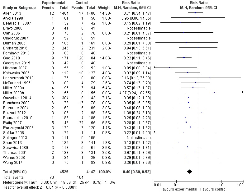
Figure 1. Forest plot summarizing complete-case analyses from systematically reviewed clinical trials of probiotics for the prevention of Clostridium difficile‐associated diarrhea (CDAD) in adults and children. Although only 4 of the 31 individual trials had statistically significant results, the pooled estimate shows a statistically and clinically signficant reduction in risk of CDAD for the studied probiotics, without statistically significant heterogeneity among the individual trials’ relative risk estimates. Note that the confidence inferval for the pooled estimate is entirely contained by all but two of the confidence intervals from the individual trials and that even the confidence intervals from these two exceptions largely contain the pooled estimate.
Reprint of Figure 3 from Joshua Z Goldenberg, Christina Yap, Lyubov Lytvyn, et al’s “ Probiotics for the prevention of Clostridium difficile‐associated diarrhea in adults and children”, published December 12, 2017 in “Cochrane Database of Systematic Reviews” by John Wiley and Sons. Copyright by John Wiley and Sons. Reprinted under one-time use license from John Wiley.
Summary
In conclusion, p values are an important component of determining whether an outcome can be deemed to be statistically significant, but this depends on the question under investigation, and is only one part of a more complete analysis. When appraising evidence for whether an intervention works, it is important to keep in mind that if one relies only on statistical inferences from individual studies, one is vulnerable to making unreliable assessments that substantially misstate the plausibility that an intervention does (or does not) have an effect. Statistical analysis cannot replace context-specific scientific judgment; both are needed to make reliable evidence appraisals.
A deeper dive into how to use p-values to assess the probability that the null hypothesis is true
A common misinterpretation of p-values is that they measure the probability that the null hypothesis is true, given the sample data. As stated above, the p-value, by itself, cannot speak to this probability, but if one is willing to supply a judgment on the prior probability that the null hypothesis is true, one can use that and the p-value to get a lower bound on the probability of interest. The compelling figure that accompanies Regina Nuzzo’s terrific Nature article on p-values and their shortcomings nicely illustrates such results for six combinations involving three example prior probabilities and p-values of 0.05 and 0.01.4 Table 1 shows posterior probabilities for those and other input combinations.
| Table 1. Plausible lower bound for the posterior (post-study) probability of the null hypothesis being true for a given prior (pre-study) probability and study p-value. Note that low p-values do not necessarily imply that the null hypothesis is unlikely to be true! | |||||||
| P-value | |||||||
| Prior Probability for Null | 0.1000 | 0.0500 | 0.0100 | 0.0050 | 0.0010 | 0.0005 | 0.0001 |
| 5% | 3.2% | 2.1% | 0.7% | 0.4% | 0.1% | 0.1% | 0.0% |
| 10% | 6.5% | 4.3% | 1.4% | 0.8% | 0.2% | 0.1% | 0.0% |
| 25% | 17.3% | 12.0% | 4.0% | 2.3% | 0.6% | 0.3% | 0.1% |
| 50% | 38.5% | 28.9% | 11.1% | 6.7% | 1.8% | 1.0% | 0.2% |
| 75% | 65.3% | 55.0% | 27.3% | 17.8% | 5.3% | 3.0% | 0.7% |
| 90% | 84.9% | 78.6% | 53.0% | 39.3% | 14.5% | 8.5% | 2.2% |
| 95% | 92.2% | 88.6% | 70.4% | 57.8% | 26.3% | 16.4% | 4.5% |
| Note: Calculations use the Bayes Factor – e p ln(p), which is shown to be a lower bound for the Bayes Factor among an appealing set of candidates, thus resulting in a plausible “lower bound” for the posterior probability that the null hypothesis is true. For example, when the prior probability is 50%, a p-value of 0.05 implies that the null hypothesis retains at least a 28.9% probability of being true. | |||||||
The calculations used in that figure and in Table 1 for converting the two inputs, a prior probability for the null hypothesis and a p-value, into a posterior probability for the null hypothesis is simply an application of a much more general formula, one that has been known for over 200 years. This formula is simple to state and remember when expressed as odds. According to Bayes Theorem, Posteriors Odds equals Prior Odds multiplied by a term we call the Likelihood Ratio. The likelihood ratio is a ratio of two conditional probabilities for the observed data, with each computed under differing hypotheses.5 [Another very widely-used application of this general formula is when physicians use the results and the operational characteristics (e.g. the sensitivity and specificity) of clinical tests to inform medical diagnoses.6] The formula uses odds not in the way that they are defined in horse racing where long-shots have high odds, but in the way that statisticians define it, as the ratio of the probability of an event to the probability of the absence of that event. To a statistician, high odds mean high probability for the event. When the probability of an event P is greater than 0, the odds are P / (1 – P). For example, if the probability of an event is 0.75 (or 75%), then the odds would be 0.75 / ( 1 – 0.75 ) = 3. If one knows the odds O, then one can find the probability P, using the equation P = O / ( 1 + O ). For example, if the odds are 4:1, or 4, then the probability is 4/5 = 0.80, and if the odds are 1:4, or 0.25, then the probability is 0.25 / 1.25 = 0.20.
In order to use this long-known formula, one has to have a way to convert the p-value into a value to use for the “Likelihood Ratio” term, which in this context is called a Bayes Factor. For the Nature article, Nuzzo used a conversion proposed in the 1990s by Thomas Sellke, M. J. Bayarri, and James O. Berger and that they eventually published in the widely read American Statistician. That conversion has an appealing statistical motivation as the minimum possible value for the Bayesian Factor among a realistic set of candidates and thus it provides a useful plausible lower bound on the Bayesian Factor for p < 1 /e ≈ 0.368, where e is the Euler number, exp(1) ≈ 2.718,7 BayesFactor = – e * p * ln(p), where ln(p) is the natural logarithm of p. (For p ≥1/e, one can use BayesFactor=1.) For example, p=0.04 would result in a BayesFactor of -exp(1) * 0.04 * ln( 0.04 ), approximately 0.35. So, if one specified that the prior probability for the null hypothesis is 50%, a toss-up, that corresponds to a prior odds of 1, then the BayesFactor for a p-value of 0.04 converts that prior odds of 1 into a posterior odds of 0.35, which corresponds to a posterior probability of 26% for the null hypothesis, substantially higher than 4%. In the analogous setting of diagnostic medicine, consider a test result that moves a physician’s suspicion for whether the patient has a disease from a pre-test value of 50% up to a post-test value of 74%. Such a result would be considered useful, but it would not be considered definitive, something for clinicians to keep in mind when they see that a study’s p-value was just under 0.05!
Another notable conversion of the p-value into a Bayes Factor was, as far as I can tell, first reported in a pioneering 1963 article in the social sciences literature that was authored by illustrious Bayesian statisticians. 8 That same Bayes Factor formula can be found clearly presented in the second5 of Steven N. Goodman’s excellent two-part set of Annals of Internal Medicine articles concerning fallacious use of p-values in evidence-based medicine. That conversion involves statistics that have an approximately normal distribution and is thus applicable to most statistics in the medical literature. That conversion reports the minimum theoretically possible value for the Bayes Factor, BayesFactormin = exp( – Z2 / 2 ), where Z is the number of standard errors the test statistic is from the null value. (Z can be estimated in Microsoft Excel by using the formula Z = NORMSINV( p ) or Z = NORMSINV( p / 2 ). For example, a two-sided p-value of 0.04 corresponds to Z ≈ -2.054 and a BayesFactormin of exp( – (-2.054 * -2.054) / 2 ) ≈ 0.121. So, if the prior probability for the null hypothesis is 50%, a p-value of 0.04 would mean that, at the minimum, the null hypothesis has a posterior probability of 0.121 / 1.21 = 10.8% of being true, substantively higher than the 4% probability that the popular misinterpretation of p-values would yield. When that factor was introduced in the 1963 article, it was noted by the authors as not being one that would be realistically attained by any study, as it would involve an impossibly lucky guess for the best possible prior probability to use, but it is still useful mathematically because it results in a theoretical minimum for the posterior probability that the null hypothesis is true. In mathematics, we routinely use well-chose impractical scenarios to define the limits for what is practically possible. Given that decisionmakers want to know how probable the null hypothesis remains in light of the study data, it is helpful to know the minimum possible theoretical value for it. Table 2 shows these posterior probabilities for the same inputs used above in Table 1. Notably, a p-value of 0.05 may not even be enough to make the null hypothesis less likely than not!
| P-value | |||||||
| Prior Probability for Null | 0.1000 | 0.0500 | 0.0100 | 0.0050 | 0.0010 | 0.0005 | 0.0001 |
| 5% | 1.3% | 0.8% | 0.2% | 0.1% | 0.0% | 0.0% | 0.0% |
| 10% | 2.8% | 1.6% | 0.4% | 0.2% | 0.0% | 0.0% | 0.0% |
| 25% | 7.9% | 4.7% | 1.2% | 0.6% | 0.1% | 0.1% | 0.0% |
| 50% | 20.5% | 12.8% | 3.5% | 1.9% | 0.4% | 0.2% | 0.1% |
| 75% | 43.7% | 30.5% | 9.8% | 5.5% | 1.3% | 0.7% | 0.2% |
| 90% | 69.9% | 56.9% | 24.6% | 14.9% | 3.9% | 2.1% | 0.5% |
| 95% | 83.1% | 73.6% | 40.8% | 27.0% | 7.8% | 4.3% | 1.0% |
| Note: For 2-sided p-values based on approximately normally distributed test statistics, using the mathematically lowest theoretically possible Bayesian Factor,5,8 thus ensuring the lowest possible value for the posterior probability for the null hypothesis. Although these lower bonds would never be attained in any realistic application, this table is useful in showing the smallest null hypothesis probability that is even theoretically possible. Note that even with a p-value of 0.05, the posterior probability for the null hypothesis may still be high. | |||||||
References
- Wasserstein RL, Lazar NA. The ASA Statement on p-Values: Context, Process, and Purpose. The American Statistician. 2016;70(2):129-133.
- Goodman SN. Toward evidence-based medical statistics. 1: The P value fallacy. Annals of Internal Medicine. 1999;130(12):995-1004.
- Goldenberg JZ, Yap C, Lytvyn L, et al. Probiotics for the prevention of Clostridium difficile-associated diarrhea in adults and children. Cochrane Database Syst Rev. 2017;12:CD006095.
- Nuzzo R. Statistical Errors. Nature. 2014;506(7487):150-152.
- Goodman SN. Toward evidence-based medical statistics. 2: The Bayes factor. Annals of Internal Medicine. 1999;130(12):1005-1013.
- Deeks JJ, Altman DG. Diagnostic tests 4: likelihood ratios. Bmj. 2004;329(7458):168-169.
- Sellke T, Bayarri MJ, Berger JO. Calibration of p values for testing precise null hypotheses. Am Stat. 2001;55(1):62-71.
- Edwards W, Lindman H, Savage LJ. Bayesian Statistical-Inference for Psychological-Research. Psychol Rev. 1963;70(3):193-242.


